
2D VSP kinematic inversion
Introduction
Determination of seismic velocities and geometry of reflecting boundaries in the borehole environment is one of the essential tasks solved by VSP method because the accuracy of velocity model used for further processing is a basis for help provide the reliable data of high quality. Determination of kinematic medium characteristics using VSP data usually includes construction of an initial approximation of velocity model and a following iterative process of the hodograph optimized inversion (Рыжиков, Троян, 1994). As a result, such model parameters are selected to help provide the best coincidence between observed and model VSP travel times. The problem of making more precise a seismic boundary structure is successfully solved for the homogeneous schistose isotropic model of medium with bounds approximated by polynomials (Савин, Шехтман, 1994). The present work observes a solution of inverse kinematic task aimed at recovery of reflecting boundary geometry and also velocities and its vertical gradients of pressure and share waves. Reflecting boundary geometry is described by cubic splines. Parameter selection is accomplished with the use of the medium initial section. VSP hodographs of different types of waves such as direct wave and up and down going pressure a share waves are used in data processing.
Method
In case of media with curvilinear boundaries and non-uniform velocity distribution the problem of model parameters determination is divided into several basic phases. At the first phase the pressure wave velocities are reinstated in each of the layers with a certain accuracy using well-known layer section over all hodographs of the direct wave. It is considered the section boundaries to be straight. In this way the received zero-range approximation of the complex constructed medium is represented in the form of the horizontally schistose model. The next phase is a problem of making more precise the sectional boundary geometry with accuracy to polynomial of low degree (under the 4th degree) and also velocities and its vertical gradients of pressure and share waves within medium layers. Making more precise is accomplished with the use of VSP travel times of different types of waves (direct wave as well as all monotype primaries) by means of optimum minimization of the mean-square values of discrepancy of an initial and model travel times. At the final phase of medium model construction the sectional boundary geometry is made more precise in the form of cubic splines with smoothing over all hodographs of all present waves by means of a gradual addition of nodes and its optimum site selection. After making a change the reflecting boundary geometry its parameters are made more precise to the necessary degree within each of the medium layers. Selection of the reflecting boundary geometry and its parameters is accomplished by means of the modified algorithm of Hooke-Jeeves’s multidimensional optimization (Гергель et al., 2001). The model hodographs are calculated in the complex constructed media by means of algorithm of the ray tracing method (Табаков et al., 2002).
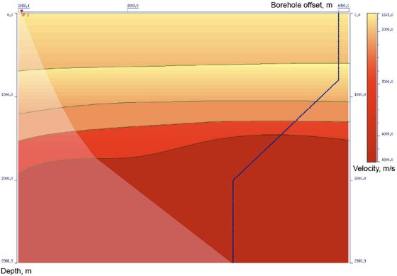
Figure 1. Initial 2D velocity model
Results
The exact velocity model is shown in Figure 1. Transparency is used for designation of shadow zone. Zero range velocity model and wave field with all laid model travel times (direct wave as well as monotype and converted primaries) is shown in Figure 2. The results of velocity model selection with polynomial boundaries over all travel times of different types of waves using well known initial layer section are represented in Figure 3. In Figure 4 the results of velocity model optimization in case of spline boundaries and the corresponding hodographs are represented. Further the mean square values of discrepancy over travel times of all used waves are shown in Figure 5. Discrepancy values are intended for the zero-range approximation model and also the models with boundaries represented by polynomials and splines. Thus, as a result of these performed calculations the received consistent velocity medium model is in accordance with expected result.
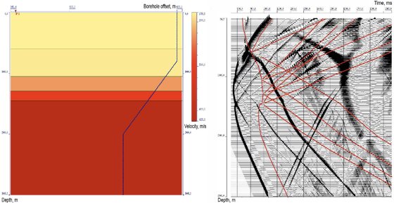
Figure 2. First approximation 1D velocity model and wavefield with modelled travel times.
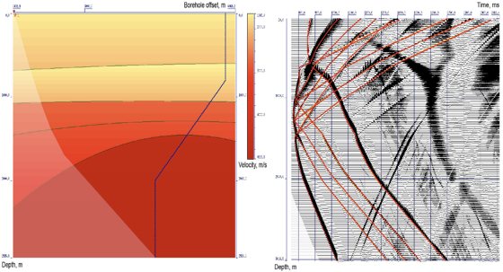
Figure 3. Velocity model with polynomial boundaries and wavefield with modelled travel times
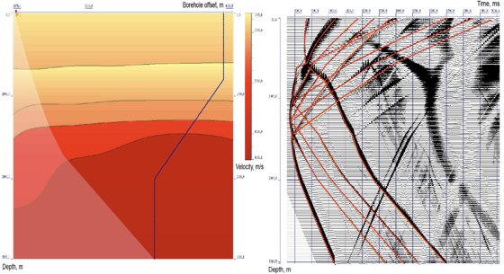
Figure 4. Velocity model with spline boundaries and wavefield with modelled travel times.
Figure 5. The mean square values of discrepancy over travel times of all used waves.
References
- Рыжиков Г.А., Троян В.Н. 1994. Томография и обратные задачи дистанционного зондирования. СПб.
- Савин И. В., Шехтман Г. А. 1994. Обратная кинематическая задача ВСП для сред с неплоскими границами раздела.
- Гергель В.П., Гришагин В.А., Городецкий С.Ю. 2001. Современные методы принятия оптимальных решений. Нижний Новгород.
- Табаков А.А., Солтан И.Е., Решетников А.В., Решетников В.В. 2002. Динамическая декомпозиция волновых полей и реконструкция модели среды при обработке данных ВСП. Материалы научно-практической конференции «Гальперинские чтения-2002». С. 12-13.
Contact Info
- Email:[email protected]
- Location:Singapore
Status: Interested in collaboration and full-time oportunities